Risk management - Simple network with lag
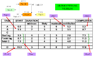
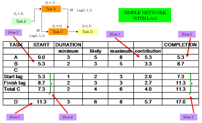
Diagram 1
Simple network with lag
The above diagram represents a spreadsheet for the second of the previous activity networks where Task C begins later than Task B due to a ‘lag’.
The spreadsheet shows the following fields:
TaskLists the task activities as described in the network.
StartThis is the start time of each task as calculated in the spreadsheet.
DurationThese are the 3 point estimates showing the MINIMUM, LIKELY and MAXIMUM.
ContributionThis is the average of the 3 point estimate values (MINIMUM + LIKELY + MAXIMUM)/3.
CompletionThis is the calculated end date or completion for each task. In the main this is the sum of the start value and the contribution, however, this is slightly more complex for activity networks where probabilities are taken into account [see complex branching].
Note 1:
As referred to above this is the sum of the minimum, likely and maximum values and divided by 3 to get the average. In the same manner as for costs it is a way of weighting the 3 point estimate.
Note 2:
The completion date is the sum of the start and the contribution values.
Note 3 and 4:
The start is 0.0 for the first task in the network. Task B naturally will start from the end date of Task A.
However, for Task C we have a lag so it doesn’t begin at the same time as Task B.
We use a 3 point estimate for the start lag (start to start) and the finish lag (finish to finish).
These are then treated in exactly the same way as for the normal task calculations.
We know that the start lag will begin at the end of Task A value = 5.3. The start lag will have a contribution of 2.0 based upon its 3 point estimate.
Therefore, the start of Task C (taking into account the start lag) will be 2.0 + 5.3 = 7.3.
In a similar fashion, we use a 3 point estimate for the finish lag (finish to finish). These are then treated in exactly the same way as for the normal task calculations.
We know that the finish lag will begin at the end of Task B value = 8.7. The finish lag will have a contribution of 2.7 based upon its 3 point estimate.
Therefore, the completion of Task C (taking into account the finish lag) will be 8.7 + 2.7 = 11.3.
As a check (Task field labelled ‘total C’) we know that Task C will begin at 7.3 (start lag completion) and the contribution derived from its 3 point estimate is 4.0.
The sum of both is 7.3 + 4.0 = 11.3.
Task D can not begin until the end of whatever is the longest task of either B or C. In this case it is Task C. So, the start of Task D is the end of Task C at a value of 11.3. The final activity network completion date will be the end of Task D which is 11.3 + 5.7 (its 3 point estimate contribution) = 17.0.
Simulation
The spreadsheet simulation will carry out perhaps 300 to 1000 iterations and each time will firstly set Task A to a value based upon its 3 point estimate.
This will lead to a completion time for Task A which will be the start time of Tasks B.
The start of Task C will be calculated based upon the Task A value and the value set for the start lag.
Each of these will, in turn, have a duration based upon their 3 point estimates (and in the case of Task C its start and finish lags) affording individual completion dates.
Eventually, there will be a value calculated for the completion date of Task D.
This final completion date will be recorded.
Over many iterations a MONTE CARLO distribution will result having a MINIMUM duration of (3 + 3 + 3) = 9 weeks and a MAXIMUM of (8 + 9 + 8) = 25 weeks.
Note the MINIMUM time will be different to the last case. This is because Task C will have a 2 week minimum duration but also a minimum of 1 week delay, giving 3 weeks in all.
The MAXIMUM time is based upon the longer of the 3 point estimate times for Task C of 6 weeks plus its longest start lag time of 3 weeks, giving 9 weeks in all.
We could also have looked at Task C from the pint of view of Task B. Its completion date is 8.7 weeks. The finish to finish lag is 2.7 weeks giving a total of 8.7 + 2.7 = 11.4 for C.
The difference from 11.3 is down to rounding to 1 decimal place.
From this data a graph of PROBABILTY versus TOTAL DURATION will be formed.
In a similar vein to the COST scenario we will be able to, for example, set a ‘total duration’ at which there is a ‘likelihood’ of 20% of it being exceeded.
The TOTAL DURATION added on to the start date of 0.0 will give the project COMPLETION DATE.
In addition, CORRELATED EVENTS could be included as for the ‘cost risk assessment’. For this one would need to identify the INDEPENDENT task and then the DEPENDANT tasks which take their lead from it according to the underlying cause.