Risk management - Complex branching part 2
Complex branching part 2
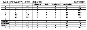
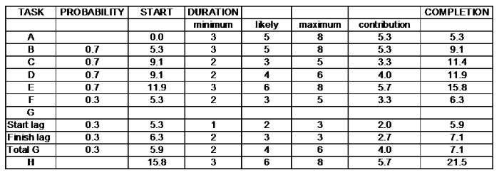
Diagram 1
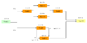
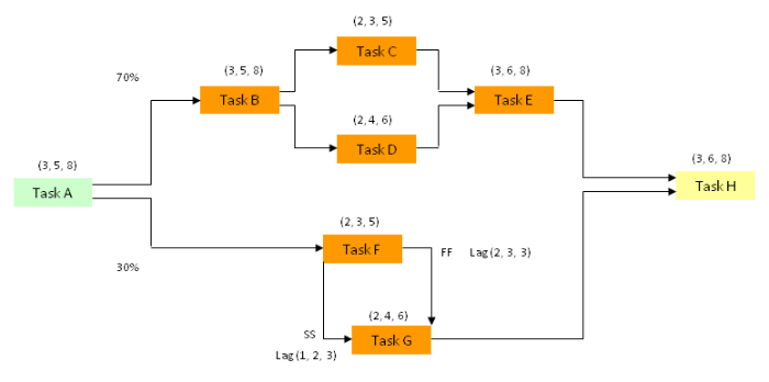
Diagram 2
In a similar fashion to the last example [see complex branching] when the upper pathway (Task B) is set to ‘1’ it will occur. When the software allows it to occur 7 times out of 10 it will have an occurrence of 70%.
Task A begins at 0.0 and its duration is 5.3 which is the start for both Task B and Task F (although this is not obvious from the way diagram 2 is drawn for convenience).
For Task B the ‘completion time’ is calculated as (probability x contribution) + the start value. That is (0.7 x 5.3) + 5.3 = 3.7 + 5.3 = 9.1 (when accurately calculated using more than one decimal place).
Similarly, Task C and Task D both start at the completion of Task B which is 9.1. Again, these both have a probability of occurring of 70% and their completion times are calculated as:
Task C: (0.7 x 3.3) + 9.1 = 2.3 + 9.1 = 11.4
Task D: (0.7 x 4.0) + 9.1 = 2.8 + 9.1 = 11.9
Again, Task E has a 70% chance of occurrence, giving:
Task E: (0.7 x 5.7) + 11.9 = 4.0 + 11.9 = 15.8 (when accurately calculated using more than one decimal place).
So, Task E will complete 15.8 weeks after the start.
In a similar fashion, when the lower pathway (Task F) is set to ‘1’ this will occur instead of Task B. When the software allows it to occur 3 times out of 10 it will have an occurrence of 30%.
For Task F: (0.3 x 3.3) + 5.3 = 1.0 + 5.3 = 6.3
In this case, for Task G, we have a start to start lag and a finish to finish lag.
The end durations for the start to start lag and a finish to finish lag are calculated as in the earlier example.
The start lag begins at 5.3.
Start lag: (0.3 x 2.0) + 5.3 = 0.6 + 5.3 = 5.9
Finish lag: (0.3 x 2.7) + 6.3 = 0.8 + 6.3 = 7.1
Overall for Task G: (0.3 x 4.0) + 5.9 = 1.2 + 5.9 = 7.1
Therefore, Task E will finish later than Task G and is used as the start for Task H.
Task H: 15.8 + 5.7 = 21.5
Simulation
The spreadsheet simulation will carry out perhaps 300 to 1000 iterations and each time will firstly set Task A to a value based upon its 3 point estimate.
This will lead to a completion time for Task A which will be the start time of Tasks B and F.
Each of these will in turn have a duration based upon their 3 point estimates affording individual completion dates.
Eventually, there will be a value calculated for the completion date of Task H.
This final completion date will be recorded.
Over many iterations a MONTE CARLO distribution will result having a MINIMUM duration of (3 + [2 +1] + 3) = 9 weeks and a MAXIMUM of (8 + [8 + 6 + 8] +8) = 38 weeks.
The MINIMUM time is based upon the minimum for Tasks G (2 weeks + 1 week lag) and Task A and H, giving 9 weeks.
The MAXIMUM time is based upon the maxima for Tasks A, B and Task D (6 weeks) and Task E and H giving 38 weeks.
From this data a graph of PROBABILITY versus TOTAL DURATION will be formed.
In a similar vein to the ‘cost’ scenario we will be able to, for example, set a ‘total duration’ at which there is a ‘likelihood’ of 20% of it being exceeded.
The TOTAL DURATION added on to the start date of 0.0 will give the project COMPLETION DATE.
In addition, CORRELATED EVENTS could be included as for the ‘cost risk assessment’. For this one would need to identify the INDEPENDENT task and then the DEPENDANT tasks which take their lead from it according to the underlying cause.
As in the previous example, when looking at the spreadsheet and the mechanism for the iteration it is worth remembering that the probability values will not actually be seen as 0.7 or 0.3 (although the software might possibly be set to show this).
This is because the software doesn’t actually provide a value of 0.7. In effect, it will give the pathway through Task B a value of ‘1’ or ‘0’ (ON or OFF). When the value is ‘1’ the software will ignore the alternative pathway (which will be set to ‘0’) and set a value for Task B. This will lead to a calculation of the total duration for the completion of Task H.
In practice the software will set this pathway probability value to ‘1’ approximately 7 times in every 10 iterations, leading to a 70% chance of occurrence.
Naturally, the other pathway (through Task F) will be set in the opposite manner to get a 30% chance of occurrence.