Risk management - Monte Carlo risk distribution
Monte Carlo risk distribution
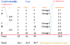
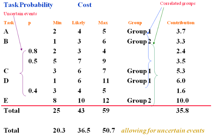
The earlier example (diagram 2 below) for tasks A, B, C, D and E was:
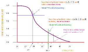
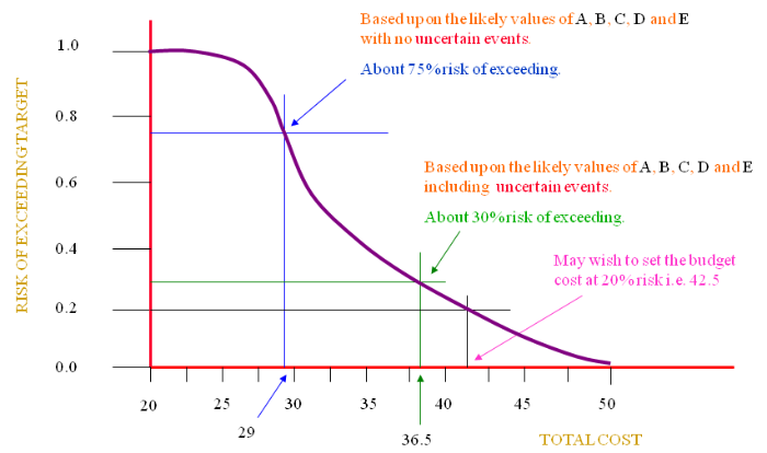
If we look at the above graph (diagram 1, not accurate but designed to give an idea of the principal) we can see several points.
Using the data seen previously (diagram 2) the SUM of the most LIKELY values NOT taking into account an uncertain values = 29. We can see from the graph that this has approximately a 75% chance of being exceeded. In other words there is a very strong possibility that if 29 was set as the budget it would be exceeded.
This reflects what we might expect in the real world where uncertain events occur. In other words, if we don’t bother to consider potential uncertain events it is highly likely the budget will be exceeded.
If we look at the data for the SUM of the most LIKELY values that also include the uncertain events the value increases to = 36.5.
This has only 30% risk of being exceeded. This is much better than the precious 75% but could still prove too low a cost to set as a budget.
It is quite typical to set the budget at a RISK of exceeding the target at 20%. In this case, the value would be = 42.5.
Remember though that the graph is not a true representation of the values and exists only for demonstration purposes.
Task (work package) contributions can be derived in other ways [see Multiple variables].


