Risk management - Multiple probability branching part 2
Multiple probability branching part 2
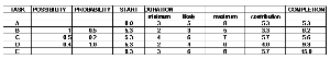
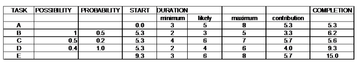
Diagram 1
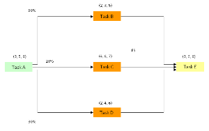
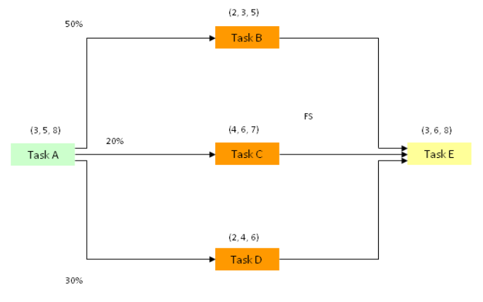
Diagram 2
In order to see what happens when we have a triple branching point we need to introduce another field to help calculate the task durations and the end points.
In the previous examples [see multiple probability branching] where we just had 2 branches we only needed to use the ‘PROBABILITY’ field which was factored in by multiplying the contribution by it and then adding it to the start value.
Let us consider what might happen in the case of the triple branching example.
We have several scenarios.
When the iterations are carried out for the Monte Carlo distribution and Task A has been set a value then Task B is possible.
If Task B occurs then Tasks C and D do not occur.
If Task B does not occur and Task C occurs then Task D can not occur.
Lastly, if Tasks B and C do not occur then Task D MUST OCCUR.
There is a relationship between each of the 3 tasks B, C and D.
The mathematics to describe this relationship can be pretty complex but the use of ‘possibility’ and ‘probability’ can simplify it slightly.
Because Task B is the first pathway in the iteration there is always a ‘possibility’ that it can occur so it will have a value of ‘1’.
Naturally, depending on what happens with Task B, Task C may or may not occur so its ‘possibility’ of happening will be less than ‘1’.
The exact ‘possibility’ of Task C will be:
The POSSIBILITY OF TASK B x (1 – PROBABILITY OF TASK B) = 1 x (1 – 0.5) = 1 x 0.5 = 0.5.
In a similar fashion, Task D can only happen when Tasks B and C do not occur.
The exact ‘possibility’ of Task D will be:
The POSSIBILITY OF TASK C x (1 – PROBABILITY OF TASK C) = 0.5 x (1 – 0.2) = 0.5 x 0.8 = 0.4.
The probability of Task D occurring is not 0.3 (for 30%) but 1.0 (100%). This is tricky!
If the iteration has got to considering Task D then it must mean that all the others in the series (in this case Tasks B and C) did not occur so it must be 100% certain to occur.
It is therefore given as 1.0.
The overall probability of any Task happening is the POSSIBILITY x PROBABILITY.
For each task this would be:
Task B = 1 x 0.5 = 0.5
Task C = 0.5 x 0.2 = 0.1
Task D = 0.4 x 1.0 = 0.4
These values 0.5 + 0.1 + 0.4 = 1.0
They should add up to 1.0 (100%) and this needs to be checked.
In the above example the longest of Tasks B, C and D is Task D = 9.3.
This becomes the start of Task E with a finish time of 15.0 weeks.
The need for branching more than once is uncommon but can occur.
Remember that the completion of a particular task my be influenced by external factors.
For example a meeting may drive the continuation of a task.
Other tasks may continue with little interruption externally.
Simulation
The spreadsheet simulation will carry out perhaps 300 to 1000 iterations and each time will firstly set Task A to a value based upon its 3 point estimate.
This will lead to a completion time [see 'The Complete Time Management package'] for Task A which will be the start time of Tasks B, C and D.
Each of these will in turn have a duration based upon their 3 point estimates, affording individual completion dates.
Eventually, there will be a value calculated for the completion date of Task E.
This final completion date will be recorded.
Over many iterations a MONTE CARLO distribution will result having a MINIMUM duration of (3 + [2 ] + 3) = 8 weeks and a MAXIMUM of (8 + [7] +8) = 23 weeks.
The MINIMUM time is based upon the minimum for Task B or D (2 weeks) and Task A and E, giving 8 weeks.
The MAXIMUM time is based upon the maximum for Task C (7 weeks) and Task A and E, giving 23 weeks.
From this data a graph of PROBABILITY versus TOTAL DURATION will be formed.
In a similar vein to the ‘cost’ scenario we will be able to, for example, set a ‘total duration’ at which there is a ‘likelihood’ of 20% of it being exceeded.
The TOTAL DURATION added on to the start date of 0.0 will give the project COMPLETION DATE.
In addition, CORRELATED EVENTS could be included as for the ‘cost risk assessment’. For this one would need to identify the INDEPENDENT task and then the DEPENDANT tasks which take their lead from it according to the underlying cause.
As in the previous examples, when looking at the spreadsheet and the mechanism for the iteration it is worth remembering that the probability values will not actually be seen as 0.5 for task B (although the software might possibly be set to show this). This is because the software doesn’t actually provide a value of 0.5. In effect, it will give the pathway through Task B a value of ‘1’ or ‘0’ (ON or OFF). When the value is ‘1’ the software will ignore the alternative pathways (which will be set to ‘0’) and set a value for Task B. This will lead to a calculation of the total duration for the completion of Task E. In practice the software will set this pathway probability value to ‘1’ approximately 5 times in every 10 iterations, leading to a 50% chance of occurrence.
Naturally, the other pathways will be set in the opposite manner.
Some insight into an example and some points to consider are given next [see production example].